Amazon SageMaker Data Wrangler is a UI-based data preparation tool that helps perform data analysis, preprocessing, and visualization with features to clean, transform, and prepare data faster. Data Wrangler pre-built flow templates help make data preparation quicker for data scientists and machine learning (ML) practitioners by helping you accelerate and understand best practice patterns for data flows using common datasets.
You can use Data Wrangler flows to perform the following tasks:
- Data visualization – Examining statistical properties for each column in the dataset, building histograms, studying outliers
- Data cleaning – Removing duplicates, dropping or filling entries with missing values, removing outliers
- Data enrichment and feature engineering – Processing columns to build more expressive features, selecting a subset of features for training
This post will help you understand Data Wrangler using the following sample pre-built flows on GitHub. The repository showcases tabular data transformation, time series data transformations, and joined dataset transforms. Each requires a different type of transformations because of their basic nature. Standard tabular or cross-sectional data is collected at a specific point in time. In contrast, time series data is captured repeatedly over time, with each successive data point dependent on its past values.
Let’s look at an example of how we can use the sample data flow for tabular data.
Prerequisites
Data Wrangler is an Amazon SageMaker feature available within Amazon SageMaker Studio, so we need to follow the Studio onboarding process to spin up the Studio environment and notebooks. Although you can choose from a few authentication methods, the simplest way to create a Studio domain is to follow the Quick start instructions. The Quick start uses the same default settings as the standard Studio setup. You can also choose to onboard using AWS IAM Identity Center (successor to AWS Single Sign-On) for authentication (see Onboard to Amazon SageMaker Domain Using IAM Identity Center).
Import the dataset and flow files into Data Wrangler using Studio
The following steps outline how to import data into SageMaker to be consumed by Data Wrangler:
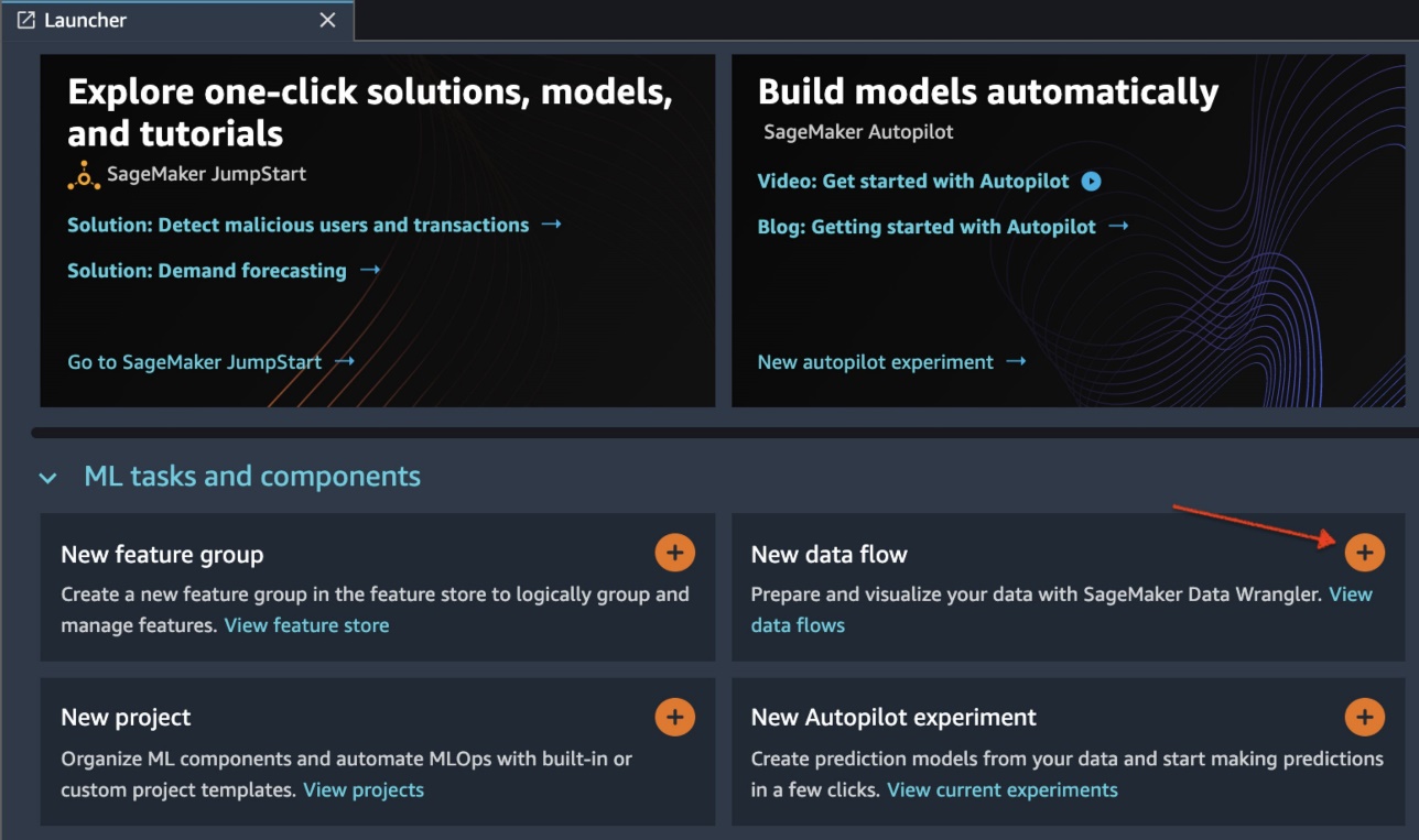
Initialize Data Wrangler via the Studio UI by choosing New data flow.
Clone the GitHub repo to download the flow files into your Studio environment.

When the clone is complete, you should be able to see the repository content in the left pane.
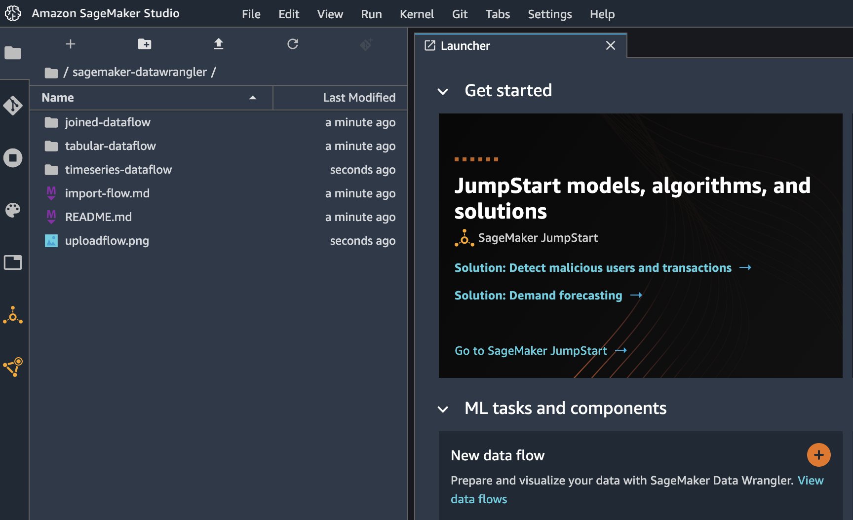
Choose the file Hotel-Bookings-Classification.flow to import the flow file into Data Wrangler.
If you use the time series or joined data flow, the flow will appear as a different name.After the flow has been imported, you should see the following screenshot. This shows us errors because we need to make sure that the flow file points to the correct data source in Amazon Simple Storage Service (Amazon S3).
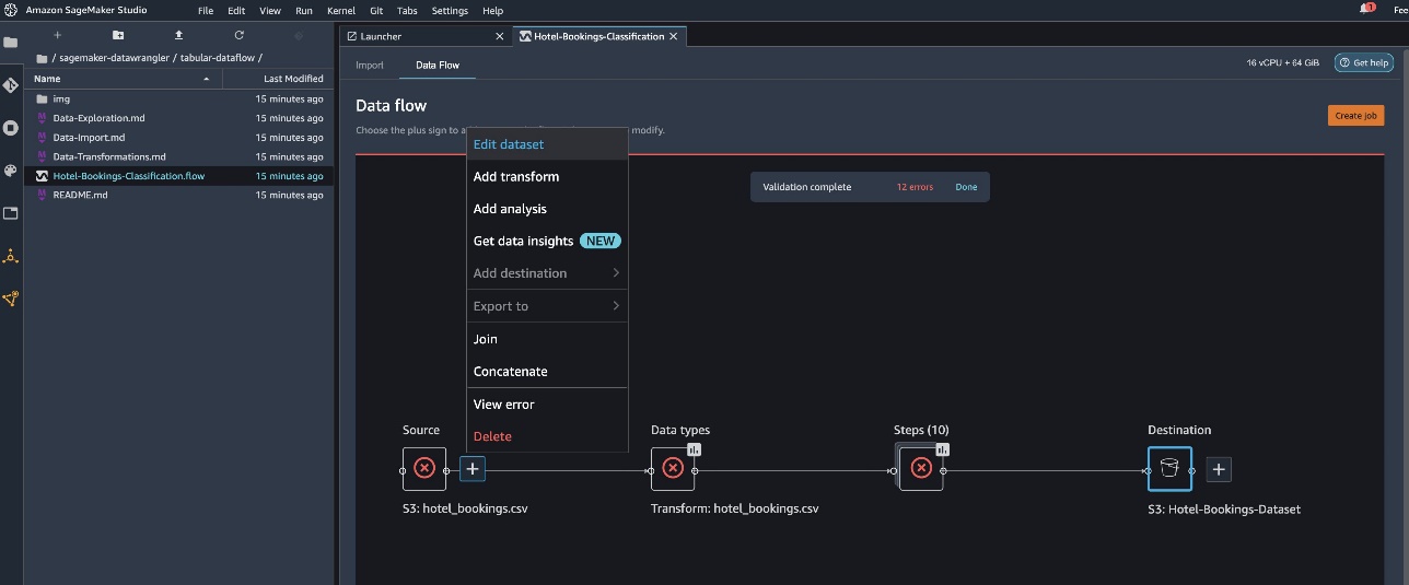
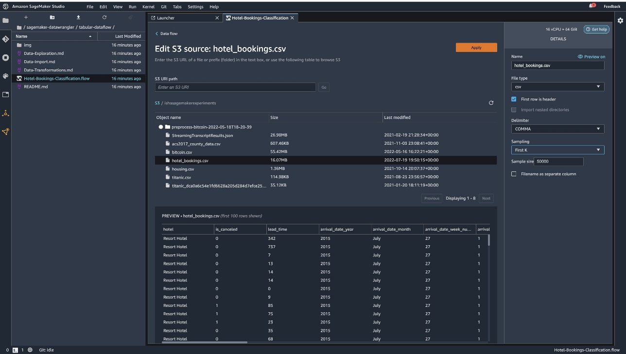
Choose Edit dataset to bring up all your S3 buckets. Next, choose the dataset hotel_bookings.csv from your S3 bucket for running through the tabular data flow.
Note that if you’re using the joined data flow, you may have to import multiple datasets into Data Wrangler
In the right pane, make sure COMMA is chosen as the delimiter and Sampling is set to First K. Our dataset is small enough to run Data Wrangler transformations on the full dataset, but we wanted to highlight how you can import the dataset. If you have a large dataset, consider using sampling. Choose Import to import this dataset to Data Wrangler.
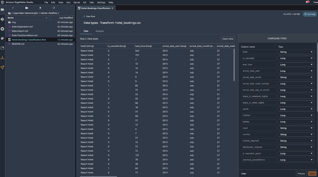
After the dataset is imported, Data Wrangler automatically validates the dataset and detects the data types. You can see that the errors have gone away because we’re pointing to the correct dataset. The flow editor now shows two blocks showcasing that the data was imported from a source and data types recognized. You can also edit the data types if needed.
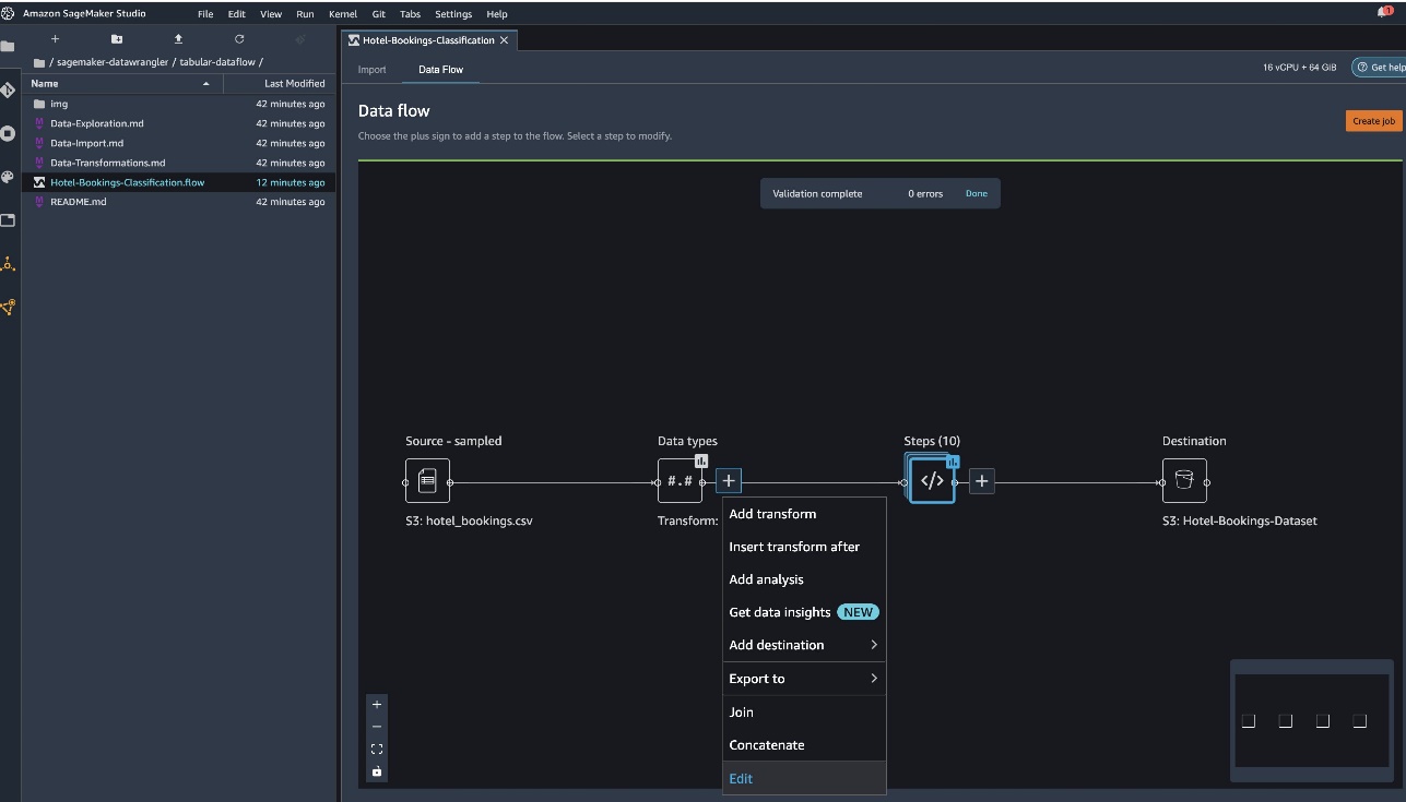
The following screenshot shows our data types.
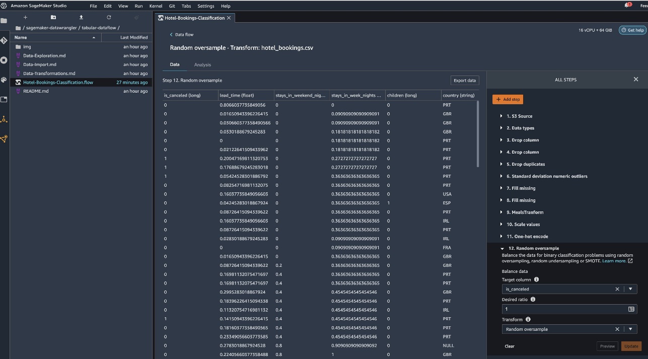
Let’s look at some of the transforms done as a part of this tabular flow. If you’re using the time series or joined data flows, check out some common transforms on the GitHub repo. We performed some basic exploratory data analysis using data insights reports that studied the target leakage and feature collinearity in the dataset, table summary analyses, and quick modeling capability. Explore the steps on the GitHub repo.
Now we drop columns based on the recommendations provided by the Data Insights and Quality Report.
- For target leakage, drop reservation_status.
- For redundant columns, drop days_in_waiting_list, hotel, reserved_room_type, arrival_date_month, reservation_status_date, babies, and arrival_date_day_of_month.
- Based on linear correlation results, drop columns arrival_date_week_number and arrival_date_year because the correlation values for these feature (column) pairs are greater than the recommended threshold of 0.90.
- Based on non-linear correlation results, drop reservation_status. This column was already marked to be dropped based on the target leakage analysis.
- Process numeric values (min-max scaling) for lead_time, stays_in_weekend_nights, stays_in_weekday_nights, is_repeated_guest, prev_cancellations, prev_bookings_not_canceled, booking_changes, adr, total_of_specical_requests, and required_car_parking_spaces.
- One-hot encode categorical variables like meal, is_repeated_guest, market_segment, assigned_room_type, deposit_type, and customer_type.
- Balance the target variable Random oversample for class imbalance.Use the quick modeling capability to handle outliers and missing values.
Export to Amazon S3
Now we have gone through the different transforms and are ready to export the data to Amazon S3. This option creates a SageMaker processing job, which runs the Data Wrangler processing flow and saves the resulting dataset to a specified S3 bucket. Follow the next steps to set up the export to Amazon S3:
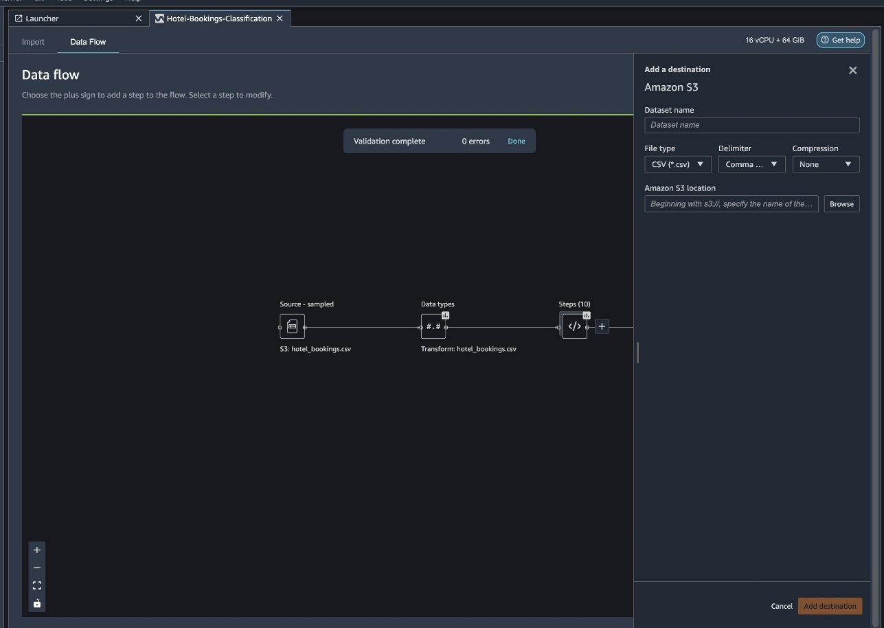
Choose the plus sign next to a collection of transformation elements and choose Add destination, then Amazon S3.
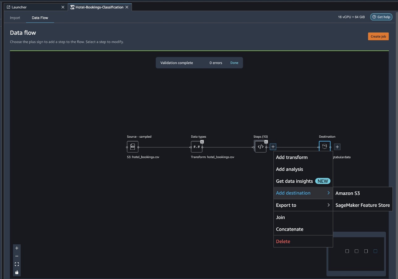
- For Dataset name, enter a name for the new dataset, for example
NYC_export. - For File type, choose CSV.
- For Delimiter, choose Comma.
- For Compression, choose None.
- For Amazon S3 location, use the same bucket name that we created earlier.
- Choose Add destination.
Choose Create job.
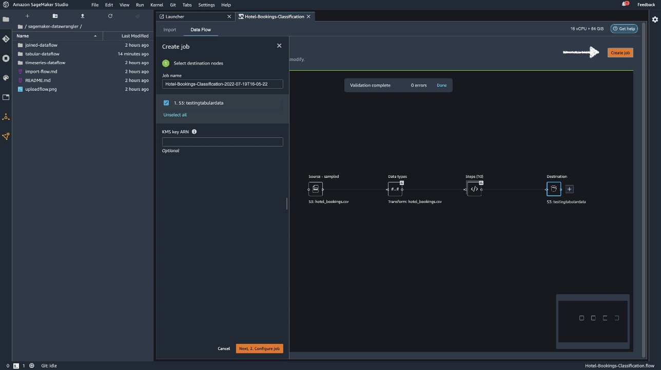
For Job name, enter a name or keep the autogenerated option and choose destination. We have only one destination, S3:testingtabulardata, but you might have multiple destinations from different steps in your workflow. Leave the KMS key ARN field empty and choose Next.
Now you have to configure the compute capacity for a job. You can keep all default values for this example.
- For Instance type, use ml.m5.4xlarge.
- For Instance count, use 2.
- You can explore Additional configuration, but keep the default settings.
- Choose Run.
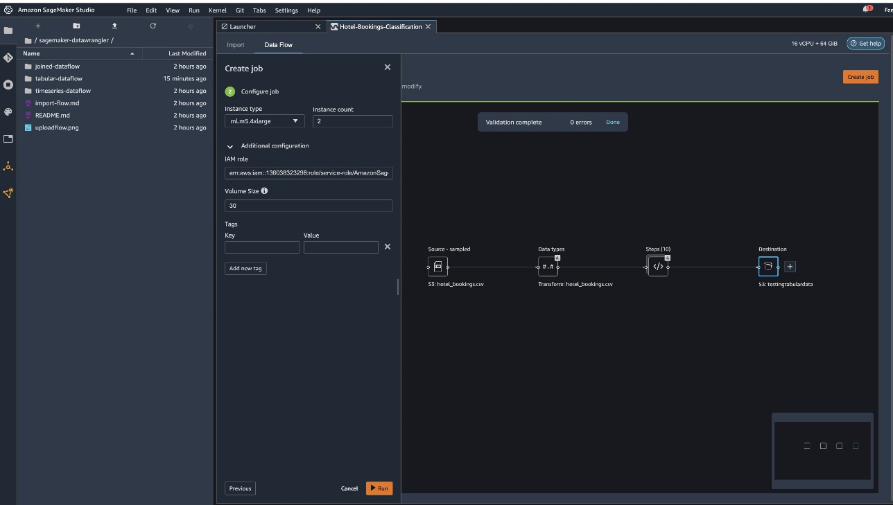
Now your job has started, and it takes some time to process 6 GB of data according to our Data Wrangler processing flow. The cost for this job will be around $2 USD, because ml.m5.4xlarge costs $0.922 USD per hour and we’re using two of them.
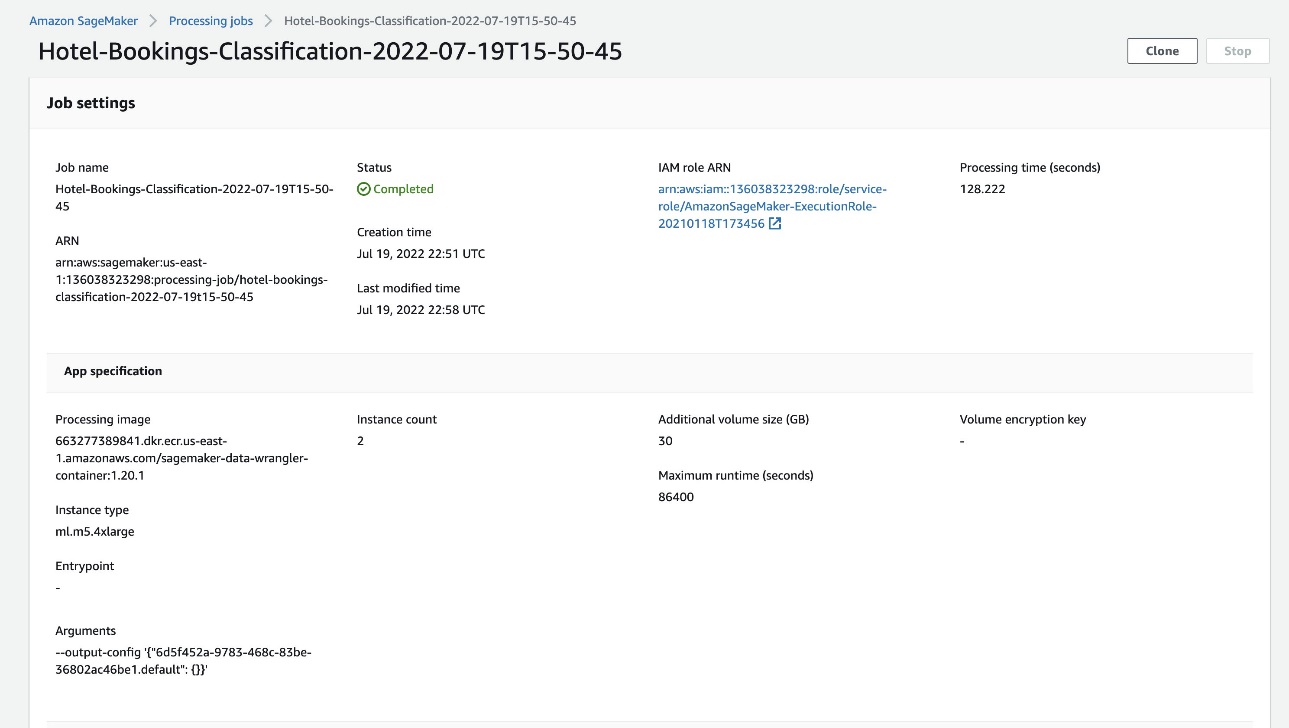
If you choose the job name, you’re redirected to a new window with the job details.
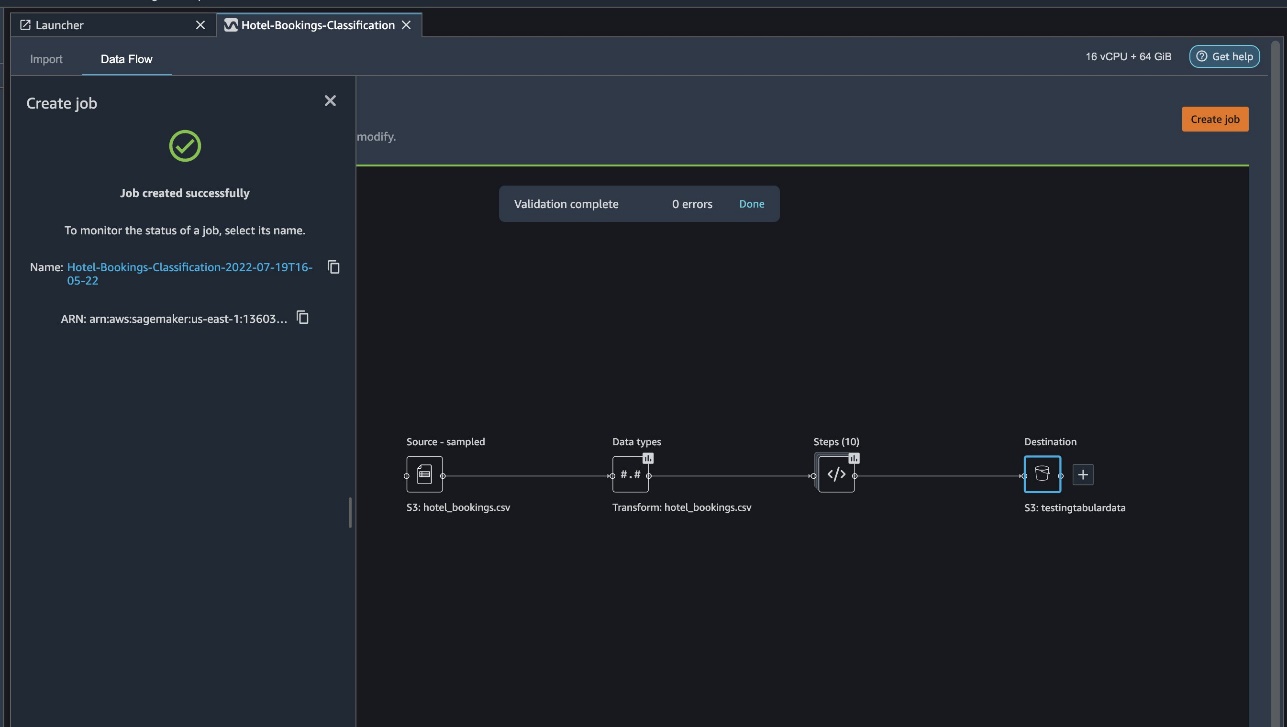
On the job details page, you can see all the parameters from the previous steps.
When the job status changes to Completed, you can also check the Processing time (seconds) value. This processing job takes around 5–10 minutes to complete.
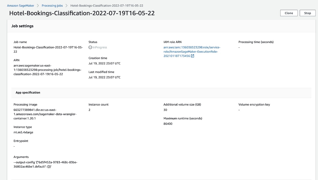
When the job is complete, the train and test output files are available in the corresponding S3 output folders. You can find the output location from the processing job configurations.
After the Data Wrangler processing job is complete, we can check the results saved in our S3 bucket. Don’t forget to update the job_name variable with your job name.
You can now use this exported data for running ML models.
Clean up
Delete your S3 buckets and your Data Wrangler flow in order to delete the underlying resources and prevent unwanted costs after you finish the experiment.
Conclusion
In this post, we showed how you can import the tabular pre-built data flow into Data Wrangler, plug it against our dataset, and export the results to Amazon S3. If your use cases require you to manipulate time series data or join multiple datasets, you can go through the other pre-built sample flows in the GitHub repo.
After you have imported a pre-built data prep workflow, you can integrate it with Amazon SageMaker Processing, Amazon SageMaker Pipelines, and Amazon SageMaker Feature Store to simplify the task of processing, sharing, and storing ML training data. You can also export this sample data flow to a Python script and create a custom ML data prep pipeline, thereby accelerating your release velocity.
We encourage you to check out our GitHub repository to get hands-on practice and find new ways to improve model accuracy! To learn more about SageMaker, visit the Amazon SageMaker Developer Guide.
About the Authors
 Isha Dua is a Senior Solutions Architect based in the San Francisco Bay Area. She helps AWS Enterprise customers grow by understanding their goals and challenges, and guides them on how they can architect their applications in a cloud-native manner while making sure they are resilient and scalable. She’s passionate about machine learning technologies and environmental sustainability.


